Other adaptive models

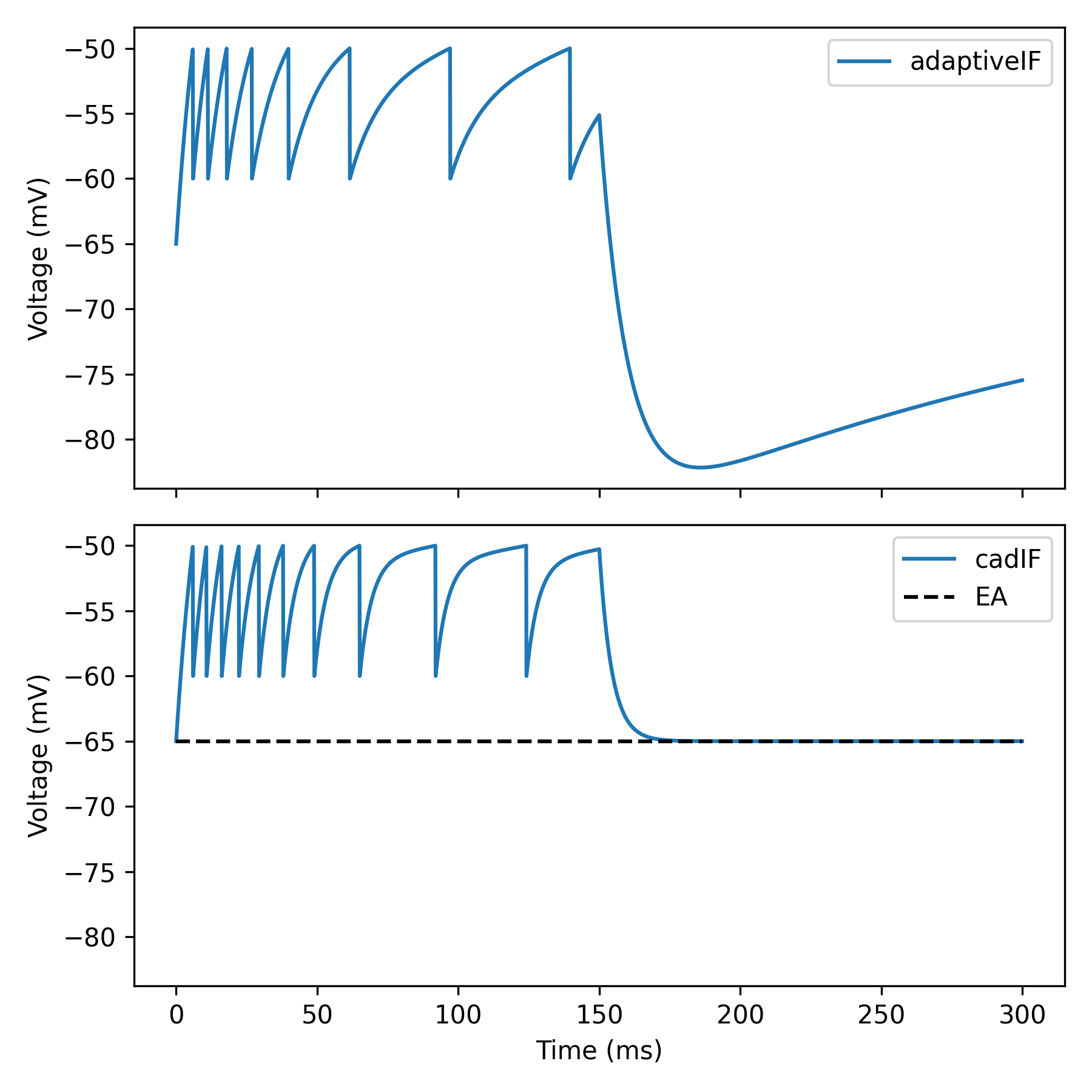
Apart from the Adaptive Exponential integrate-and-fire model (AdEx), Dendrify also supports other types of adaptive models, that can be preferred in some cases. In this example, we compare the behavior of two different adaptive models:

• The Adaptive IF model with current-based adaptation (adaptiveIF), which is simpler and faster to simulate than AdEx.

• The Conductance-based adaptive IF model (cadIF), which provides a solution to a common problem of current-based models, namely the excessive membrane hyperpolarization that can occur after high-frequency firing.

import brian2 as b
from brian2.units import Hz, ms, mV, nA, nS, pA, pF

from dendrify import PointNeuronModel

b.prefs.codegen.target = 'numpy'  # faster for simple simulations

# A point neuron model with current-based adaptation
adaptiveIF = PointNeuronModel(
    model='adaptiveIF',
    cm_abs=150*pF,
    gl_abs=15*nS,
    v_rest=-65*mV)

adaptiveIF.add_params(
    {'Vth': -50*mV,
     'tauw': 210*ms,
     'a': 0*nS,     # no subthreshold adaptation for simplicity
     'b': 60*pA,
     'Vr': -60*mV})

adaptiveIF_neuron = adaptiveIF.make_neurongroup(
    N=1,
    threshold='V>Vth',
    reset='V=Vr; w+=b',
    method='euler')

# A point neuron model with conductance-based adaptation
cadIF = PointNeuronModel(
    model='cadIF',
    cm_abs=150*pF,
    gl_abs=15*nS,
    v_rest=-65*mV)

cadIF.add_params(
    {'Vth': -50*mV,
     'tauA': 210*ms,
     'gAmax': 0*nS,     # no subthreshold adaptation for simplicity
     'delta_gA': 3*nS,
     'Vr': -60*mV,
     'EA': -65*mV})

cadIF_neuron = cadIF.make_neurongroup(
    N=1,
    threshold='V>Vth',
    reset='V=Vr; gA+=delta_gA',
    method='euler')

# Record voltages
adaptiveIF_trace = b.StateMonitor(adaptiveIF_neuron, ['V'], record=0)
cadIF_trace = b.StateMonitor(cadIF_neuron, ['V'], record=0)

# Run simulation
adaptiveIF_neuron.I_ext = 500*pA
cadIF_neuron.I_ext = 500*pA
b.run(150 * ms)
adaptiveIF_neuron.I_ext = 0*pA
cadIF_neuron.I_ext = 0*pA
b.run(150 * ms)

# Plot results
fig, axes = b.subplots(2, 1, figsize=[6, 6], sharex=True, sharey=True)
ax1, ax2 = axes
ax1.plot(adaptiveIF_trace.t / ms,
         adaptiveIF_trace[0].V / mV,
         label='adaptiveIF')
ax1.set_ylabel('Voltage (mV)')
ax1.legend()

ax2.plot(cadIF_trace.t / ms,
         cadIF_trace[0].V / mV,
         label='cadIF')
ax2.hlines(-65, 0, 300, 'k', '--', label='EA')
ax2.set_xlabel('Time (ms)')
ax2.set_ylabel('Voltage (mV)')
ax2.legend()
fig.tight_layout()
b.show()