Running simulations
In this tutorial, we are going to cover the following topics:
How to merge compartments into compartmental neuron models
How to make Dendrify and Brian interact with each other
How to run simulations of Dendrify models in Brian
Disclaimer
Below, we present a generic “toy” model developed solely for educational purposes. However, please note that its parameters and behavior have not been validated using real data. If you plan to use Dendrify in a project, we recommend calibrating the model’s parameters to suit your specific needs before applying it.
Imports & settings
import brian2 as b
import matplotlib.pyplot as plt
from brian2.units import *
from dendrify import Soma, Dendrite, NeuronModel

b.prefs.codegen.target = 'numpy' # faster for basic models and short simulations
# Plot settings
blue = '#005c94ff'
green = '#338000ff'
orange = '#ff6600ff'
notred = '#aa0044ff'
params = {
          "legend.fontsize": 10,
          "legend.handlelength": 1.5,
          "legend.edgecolor": 'inherit',
          "legend.columnspacing": 0.8,
          "legend.handletextpad": 0.5,
          "axes.labelsize": 10,
          "axes.titlesize": 11,
          "axes.spines.right": False,
          "axes.spines.top": False,
          "xtick.labelsize": 10,
          "ytick.labelsize": 10,
          'lines.markersize': 3,
          'lines.linewidth': 1.25,
          'grid.color': "#d3d3d3",
          'figure.dpi': 150,
          'axes.prop_cycle': b.cycler(color=[blue, green, orange, notred])
          }

plt.rcParams.update(params)
Create a compartmental model
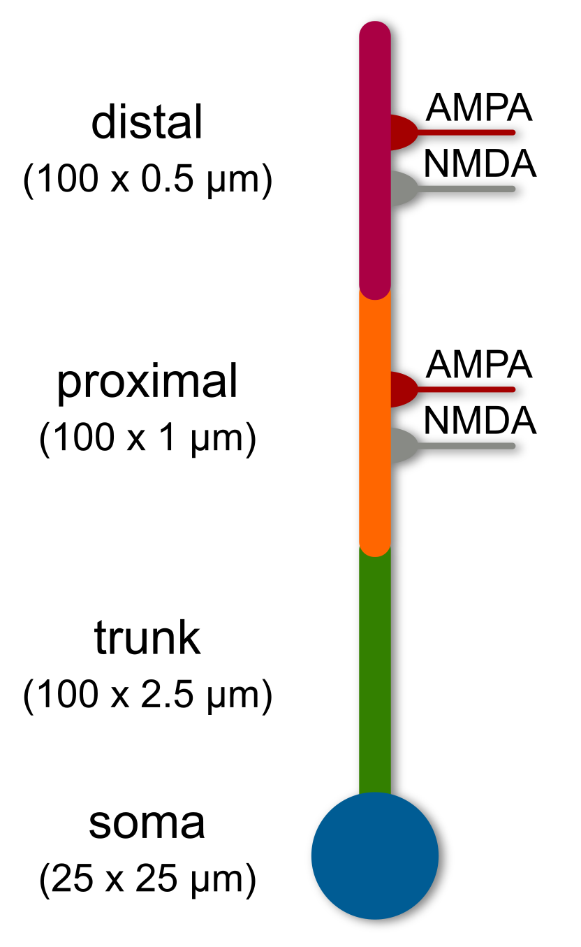
Lets try to recreate the following basic 4-compartment model:
According to the previous tutorial the code should look somethink like this:
# create soma
soma = Soma('soma', model='leakyIF', length=25*um, diameter=25*um,
            cm=1*uF/(cm**2), gl=40*uS/(cm**2),
            v_rest=-65*mV)

# create trunk
trunk = Dendrite('trunk', length=100*um, diameter=2.5*um,
                 cm=1*uF/(cm**2), gl=40*uS/(cm**2),
                 v_rest=-65*mV)

# create proximal dendrite
prox = Dendrite('prox', length=100*um, diameter=1*um,
                cm=1*uF/(cm**2), gl=40*uS/(cm**2),
                v_rest=-65*mV)
prox.synapse('AMPA', tag='pathY', g=1*nS,  t_decay=2*ms)
prox.synapse('NMDA', tag='pathY', g=1*nS,  t_decay=60*ms)

# create distal dendrite
dist = Dendrite('dist', length=100*um, diameter=0.5*um,
                cm=1*uF/(cm**2), gl=40*uS/(cm**2),
                v_rest=-65*mV)
dist.synapse('AMPA', tag='pathX', g=1*nS,  t_decay=2*ms)
dist.synapse('NMDA', tag='pathX', g=1*nS,  t_decay=60*ms)

soma.connect(trunk, g=15*nS)
trunk.connect(prox, g=6*nS)
prox.connect(dist, g=2*nS)
However, Dendrify offers a more elegant way to create a compartmental model!
# create compartments
soma = Soma('soma', model='leakyIF', length=25*um, diameter=25*um)
trunk = Dendrite('trunk', length=100*um, diameter=2.5*um)
prox = Dendrite('prox', length=100*um, diameter=1*um)
dist = Dendrite('dist', length=100*um, diameter=0.5*um)

# add AMPA/NMDA synapses
prox.synapse('AMPA', tag='pathY', g=1*nS,  t_decay=2*ms)
prox.synapse('NMDA', tag='pathY', g=1*nS,  t_decay=60*ms)
dist.synapse('AMPA', tag='pathX', g=1*nS,  t_decay=2*ms)
dist.synapse('NMDA', tag='pathX', g=1*nS,  t_decay=60*ms)

# merge compartments into a  neuron model and set its basic properties
graph = [(soma, trunk, 15*nS), (trunk, prox, 6*nS), (prox, dist, 2*nS)]
model = NeuronModel(graph, cm=1*uF/(cm**2), gl=40*uS/(cm**2),
                    v_rest=-65*mV, scale_factor=2.8, spine_factor=1.5)
The NeuronModel class not only lets you set model parameters, but also provides many useful functions that we’ll explore below.
# Print all model equations, paramaters and custom (dendritic spike) events
print(model)
OBJECT
------
<class 'dendrify.neuronmodel.NeuronModel'>


EQUATIONS
---------
dV_soma/dt = (gL_soma * (EL_soma-V_soma) + I_soma) / C_soma  :volt
I_soma = I_ext_soma + I_trunk_soma   :amp
I_ext_soma  :amp
I_trunk_soma = (V_trunk-V_soma) * g_trunk_soma  :amp

dV_trunk/dt = (gL_trunk * (EL_trunk-V_trunk) + I_trunk) / C_trunk  :volt
I_trunk = I_ext_trunk + I_prox_trunk  + I_soma_trunk   :amp
I_ext_trunk  :amp
I_soma_trunk = (V_soma-V_trunk) * g_soma_trunk  :amp
I_prox_trunk = (V_prox-V_trunk) * g_prox_trunk  :amp

dV_prox/dt = (gL_prox * (EL_prox-V_prox) + I_prox) / C_prox  :volt
I_prox = I_ext_prox + I_dist_prox  + I_trunk_prox  + I_NMDA_pathY_prox + I_AMPA_pathY_prox  :amp
I_ext_prox  :amp
I_AMPA_pathY_prox = g_AMPA_pathY_prox * (E_AMPA-V_prox) * s_AMPA_pathY_prox * w_AMPA_pathY_prox  :amp
ds_AMPA_pathY_prox/dt = -s_AMPA_pathY_prox / t_AMPA_decay_pathY_prox  :1
I_NMDA_pathY_prox = g_NMDA_pathY_prox * (E_NMDA-V_prox) * s_NMDA_pathY_prox / (1 + Mg_con * exp(-Alpha_NMDA*(V_prox/mV+Gamma_NMDA)) / Beta_NMDA) * w_NMDA_pathY_prox  :amp
ds_NMDA_pathY_prox/dt = -s_NMDA_pathY_prox/t_NMDA_decay_pathY_prox  :1
I_trunk_prox = (V_trunk-V_prox) * g_trunk_prox  :amp
I_dist_prox = (V_dist-V_prox) * g_dist_prox  :amp

dV_dist/dt = (gL_dist * (EL_dist-V_dist) + I_dist) / C_dist  :volt
I_dist = I_ext_dist + I_prox_dist  + I_NMDA_pathX_dist + I_AMPA_pathX_dist  :amp
I_ext_dist  :amp
I_AMPA_pathX_dist = g_AMPA_pathX_dist * (E_AMPA-V_dist) * s_AMPA_pathX_dist * w_AMPA_pathX_dist  :amp
ds_AMPA_pathX_dist/dt = -s_AMPA_pathX_dist / t_AMPA_decay_pathX_dist  :1
I_NMDA_pathX_dist = g_NMDA_pathX_dist * (E_NMDA-V_dist) * s_NMDA_pathX_dist / (1 + Mg_con * exp(-Alpha_NMDA*(V_dist/mV+Gamma_NMDA)) / Beta_NMDA) * w_NMDA_pathX_dist  :amp
ds_NMDA_pathX_dist/dt = -s_NMDA_pathX_dist/t_NMDA_decay_pathX_dist  :1
I_prox_dist = (V_prox-V_dist) * g_prox_dist  :amp


PARAMETERS
----------
{'Alpha_NMDA': 0.062,
 'Beta_NMDA': 3.57,
 'C_dist': 6.59734457 * pfarad,
 'C_prox': 13.19468915 * pfarad,
 'C_soma': 54.97787144 * pfarad,
 'C_trunk': 32.98672286 * pfarad,
 'EL_dist': -65. * mvolt,
 'EL_prox': -65. * mvolt,
 'EL_soma': -65. * mvolt,
 'EL_trunk': -65. * mvolt,
 'E_AMPA': 0. * volt,
 'E_Ca': 136. * mvolt,
 'E_GABA': -80. * mvolt,
 'E_K': -89. * mvolt,
 'E_NMDA': 0. * volt,
 'E_Na': 70. * mvolt,
 'Gamma_NMDA': 0,
 'Mg_con': 1.0,
 'gL_dist': 263.8937829 * psiemens,
 'gL_prox': 0.52778757 * nsiemens,
 'gL_soma': 2.19911486 * nsiemens,
 'gL_trunk': 1.31946891 * nsiemens,
 'g_AMPA_pathX_dist': 1. * nsiemens,
 'g_AMPA_pathY_prox': 1. * nsiemens,
 'g_NMDA_pathX_dist': 1. * nsiemens,
 'g_NMDA_pathY_prox': 1. * nsiemens,
 'g_dist_prox': 2. * nsiemens,
 'g_prox_dist': 2. * nsiemens,
 'g_prox_trunk': 6. * nsiemens,
 'g_soma_trunk': 15. * nsiemens,
 'g_trunk_prox': 6. * nsiemens,
 'g_trunk_soma': 15. * nsiemens,
 't_AMPA_decay_pathX_dist': 2. * msecond,
 't_AMPA_decay_pathY_prox': 2. * msecond,
 't_NMDA_decay_pathX_dist': 60. * msecond,
 't_NMDA_decay_pathY_prox': 60. * msecond,
 'w_AMPA_pathX_dist': 1.0,
 'w_AMPA_pathY_prox': 1.0,
 'w_NMDA_pathX_dist': 1.0,
 'w_NMDA_pathY_prox': 1.0}


EVENTS
------
[]


EVENT CONDITIONS
----------------
{}
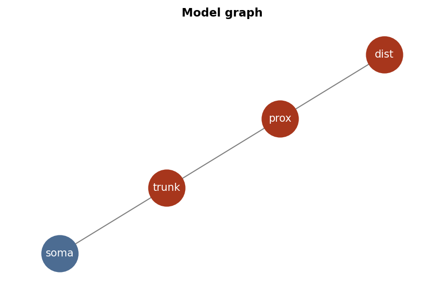
# Plot a graphical representation of the model (requires networkx to be installed)
model.as_graph()
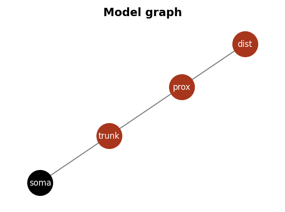
# Plot a graphical representation of the model with custom settings
model.as_graph(figsize=[4,3], scale_nodes=0.5, fontsize=8, color_soma='black')
Dendrify meets Brian
A NeuronModel allows you to directly create a Brian NeuronGroup. For more information, see the docs.
neuron, ap_reset = model.make_neurongroup(1, method='euler', threshold='V_soma > -40*mV',
                                reset='V_soma = 40*mV',
                                second_reset= 'V_soma=-55*mV',
                                spike_width = 0.5*ms,
                                refractory=4*ms)
To simulate a more realistic somatic action potential shape, a double reset mechanism can be applied. In this setup, the first reset is set to a high value (e.g., 40 mV) and the second reset to a lower value (e.g., -55 mV). The second reset is triggered after a certain time (e.g., 0.5 ms) to simulate the hyperpolarization phase of the action potential. This can be achieved by setting the second_reset parameter in the make_neurongroup function. The spike_width parameter can be used to
define the duration of the hyperpolarization phase. The refractory parameter can be used to define the refractory period of the neuron.
IMPORTANT: When a double reset mechanism is used, the make_neurongroup function returns a second object apart from the NeuronGroup that should be included in the Brian network.
# Set a monitor to record the voltages of all compartments
voltages = ['V_soma', 'V_trunk', 'V_prox', 'V_dist']
M = b.StateMonitor(neuron, voltages, record=True)
Run simulation and plot results
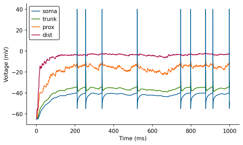
net = b.Network(neuron, ap_reset, M)  # organize everythink into a network
net.run(10*ms)  # no input
neuron.I_ext_soma = 200*pA
net.run(100*ms)  # 200 pA injected at the soma for 100 ms
neuron.I_ext_soma = 0*pA
net.run(60*ms) # run another 60 ms without any input
# Plot voltages
fig, ax = plt.subplots(figsize=(7, 4))
ax.plot(M.t/ms, M.V_soma[0]/mV, label='soma')
ax.plot(M.t/ms, M.V_trunk[0]/mV, label='trunk')
ax.plot(M.t/ms, M.V_prox[0]/mV, label='prox')
ax.plot(M.t/ms, M.V_dist[0]/mV, label='dist')
ax.set_xlabel('Time (ms)')
ax.set_ylabel('Voltage (mV)')
ax.legend(loc='best');

# Zoom in
fig, ax = plt.subplots(figsize=(7, 4))
ax.plot(M.t/ms, M.V_soma[0]/mV, label='soma')
ax.plot(M.t/ms, M.V_trunk[0]/mV, label='trunk')
ax.plot(M.t/ms, M.V_prox[0]/mV, label='prox')
ax.plot(M.t/ms, M.V_dist[0]/mV, label='dist')
ax.set_xlabel('Time (ms)')
ax.set_ylabel('Voltage (mV)')
ax.set_xlim(left=40, right=80)
ax.legend(loc='best');

The dendritic voltage fluctuations following somatic action potentials are due to the electrical coupling between these compartments. These are not backpropagating dSpikes, as they are not yet included in the model.
A network with random input
b.start_scope() # clear previous runs

# First create 2 input groups
inputX = b.PoissonGroup(50, 10*Hz) # 50 neurons firing at 10 Hz
inputY = b.PoissonGroup(50, 10*Hz) # 50 neurons firing at 10 Hz

# And a NEWronGroup (I am so funny)
group, ap_reset = model.make_neurongroup(100, method='euler', threshold='V_soma > -40*mV',
                                reset='V_soma = 40*mV',
                                second_reset= 'V_soma=-55*mV',
                                spike_width = 0.5*ms,
                                refractory=4*ms)
# Let's remember how model equations look like:
print(dist.equations)
dV_dist/dt = (gL_dist * (EL_dist-V_dist) + I_dist) / C_dist  :volt
I_dist = I_ext_dist + I_NMDA_pathX_dist + I_AMPA_pathX_dist  :amp
I_ext_dist  :amp
I_AMPA_pathX_dist = g_AMPA_pathX_dist * (E_AMPA-V_dist) * s_AMPA_pathX_dist * w_AMPA_pathX_dist  :amp
ds_AMPA_pathX_dist/dt = -s_AMPA_pathX_dist / t_AMPA_decay_pathX_dist  :1
I_NMDA_pathX_dist = g_NMDA_pathX_dist * (E_NMDA-V_dist) * s_NMDA_pathX_dist / (1 + Mg_con * exp(-Alpha_NMDA*(V_dist/mV+Gamma_NMDA)) / Beta_NMDA) * w_NMDA_pathX_dist  :amp
ds_NMDA_pathX_dist/dt = -s_NMDA_pathX_dist/t_NMDA_decay_pathX_dist  :1
Each synaptic equation includes a gate variable in the form 's_<channel>_<tag>_<compartment>', which is accessed by Brian’s Synapses objects to define the effect of presynaptic neuron activation on postsynaptic targets. In the code below, we increase the gate variable by one unit when a presynaptic neuron is activated. Otherwise, the variable decays exponentially according to the specified channel time constants.
# Define what happens when a presynaptic spike arrives at the synapse
synX = b.Synapses(inputX, group,
                  on_pre='s_AMPA_pathX_dist += 1; s_NMDA_pathX_dist += 1')
synY = b.Synapses(inputY, group,
                  on_pre='s_AMPA_pathY_prox += 1; s_NMDA_pathY_prox += 1')

# This is the actual connection part
synX.connect(p=0.5) # 50% of the inputs X connect to the group
synY.connect(p=0.5) # 50% of the inputs Y connect to the group
# Set spike and voltage monitors
S = b.SpikeMonitor(group)
voltages = ['V_soma', 'V_trunk', 'V_prox', 'V_dist']
M = b.StateMonitor(group, voltages, record=True)

# Run simulation
net = b.Network(group, ap_reset, synX, synY, S)
b.run(1000*ms)

# Plot spiketimes
fig, ax = plt.subplots(figsize=(7, 4))
ax.plot(S.t/ms, S.i, '.')
ax.set_xlabel('Time (ms)')
ax.set_ylabel('Neuron index');
# Plot voltages
fig, ax = plt.subplots(figsize=(7, 4))
ax.plot(M.t/ms, M.V_soma[0]/mV, label='soma', zorder=3)
ax.plot(M.t/ms, M.V_trunk[0]/mV, label='trunk')
ax.plot(M.t/ms, M.V_prox[0]/mV, label='prox')
ax.plot(M.t/ms, M.V_dist[0]/mV, label='dist')
ax.set_xlabel('Time (ms)')
ax.set_ylabel('Voltage (mV)')
ax.legend(loc='best');

Playing with dSpikes
In the previous model, all dendritic compartments were passive, meaning they couldn’t generate dendritic spikes. Now, let’s explore how Dendrify enables the modeling of active dendrites and how dendritic spiking influences neuronal output.
b.start_scope() # clear previous runs

# Add channels of the same type to compartments
dist.dspikes('dSpike', g_rise=3.7*nS, g_fall=2.4*nS)
prox.dspikes('dSpike', g_rise=9*nS, g_fall=5.7*nS)
trunk.dspikes('dSpike', g_rise=22*nS, g_fall=14*nS)
In the code above, 'dSpike' is an arbitrary, user-defined name. Using the same name across all compartments ensures they share a consistent spiking mechanism that can be calibrated uniformly (see below). It’s also possible to include multiple types of dendritic spikes, even within the same compartment, as long as each has a unique name. The parameters g_rise and g_fall define the conductances for the rising and falling phases of the dendritic spike, respectively, and are specific to
each compartment.
model = NeuronModel(graph, cm=1*uF/(cm**2), gl=40*uS/(cm**2),
                    v_rest=-65*mV, r_axial=150*ohm*cm,
                    scale_factor=2.8, spine_factor=1.5)

# After the a model is created, we can calibrate the behavior of the various dendritic spiking mechanisms
model.config_dspikes('dSpike', threshold=-35*mV,
                     duration_rise=1.2*ms, duration_fall=2.4*ms,
                     offset_fall=0.2*ms, refractory=5*ms,
                     reversal_rise='E_Na', reversal_fall='E_K') # Used the reversal potentials of Na and K for more realistic behavior
print(model)
OBJECT
------
<class 'dendrify.neuronmodel.NeuronModel'>


EQUATIONS
---------
dV_soma/dt = (gL_soma * (EL_soma-V_soma) + I_soma) / C_soma  :volt
I_soma = I_ext_soma + I_trunk_soma   :amp
I_ext_soma  :amp
I_trunk_soma = (V_trunk-V_soma) * g_trunk_soma  :amp

dV_trunk/dt = (gL_trunk * (EL_trunk-V_trunk) + I_trunk) / C_trunk  :volt
I_trunk = I_ext_trunk + I_prox_trunk  + I_soma_trunk  + I_rise_dSpike_trunk + I_fall_dSpike_trunk  :amp
I_ext_trunk  :amp
I_rise_dSpike_trunk = g_rise_dSpike_trunk * (E_rise_dSpike-V_trunk)  :amp
I_fall_dSpike_trunk = g_fall_dSpike_trunk * (E_fall_dSpike-V_trunk)  :amp
g_rise_dSpike_trunk = g_rise_max_dSpike_trunk * int(t_in_timesteps <= spiketime_dSpike_trunk + duration_rise_dSpike_trunk) * gate_dSpike_trunk :siemens
g_fall_dSpike_trunk = g_fall_max_dSpike_trunk * int(t_in_timesteps <= spiketime_dSpike_trunk + offset_fall_dSpike_trunk + duration_fall_dSpike_trunk) * int(t_in_timesteps >= spiketime_dSpike_trunk + offset_fall_dSpike_trunk) *  gate_dSpike_trunk :siemens
spiketime_dSpike_trunk  :1
gate_dSpike_trunk  :1
I_soma_trunk = (V_soma-V_trunk) * g_soma_trunk  :amp
I_prox_trunk = (V_prox-V_trunk) * g_prox_trunk  :amp

dV_prox/dt = (gL_prox * (EL_prox-V_prox) + I_prox) / C_prox  :volt
I_prox = I_ext_prox + I_dist_prox  + I_trunk_prox  + I_rise_dSpike_prox + I_fall_dSpike_prox + I_NMDA_pathY_prox + I_AMPA_pathY_prox  :amp
I_ext_prox  :amp
I_AMPA_pathY_prox = g_AMPA_pathY_prox * (E_AMPA-V_prox) * s_AMPA_pathY_prox * w_AMPA_pathY_prox  :amp
ds_AMPA_pathY_prox/dt = -s_AMPA_pathY_prox / t_AMPA_decay_pathY_prox  :1
I_NMDA_pathY_prox = g_NMDA_pathY_prox * (E_NMDA-V_prox) * s_NMDA_pathY_prox / (1 + Mg_con * exp(-Alpha_NMDA*(V_prox/mV+Gamma_NMDA)) / Beta_NMDA) * w_NMDA_pathY_prox  :amp
ds_NMDA_pathY_prox/dt = -s_NMDA_pathY_prox/t_NMDA_decay_pathY_prox  :1
I_rise_dSpike_prox = g_rise_dSpike_prox * (E_rise_dSpike-V_prox)  :amp
I_fall_dSpike_prox = g_fall_dSpike_prox * (E_fall_dSpike-V_prox)  :amp
g_rise_dSpike_prox = g_rise_max_dSpike_prox * int(t_in_timesteps <= spiketime_dSpike_prox + duration_rise_dSpike_prox) * gate_dSpike_prox :siemens
g_fall_dSpike_prox = g_fall_max_dSpike_prox * int(t_in_timesteps <= spiketime_dSpike_prox + offset_fall_dSpike_prox + duration_fall_dSpike_prox) * int(t_in_timesteps >= spiketime_dSpike_prox + offset_fall_dSpike_prox) *  gate_dSpike_prox :siemens
spiketime_dSpike_prox  :1
gate_dSpike_prox  :1
I_trunk_prox = (V_trunk-V_prox) * g_trunk_prox  :amp
I_dist_prox = (V_dist-V_prox) * g_dist_prox  :amp

dV_dist/dt = (gL_dist * (EL_dist-V_dist) + I_dist) / C_dist  :volt
I_dist = I_ext_dist + I_prox_dist  + I_rise_dSpike_dist + I_fall_dSpike_dist + I_NMDA_pathX_dist + I_AMPA_pathX_dist  :amp
I_ext_dist  :amp
I_AMPA_pathX_dist = g_AMPA_pathX_dist * (E_AMPA-V_dist) * s_AMPA_pathX_dist * w_AMPA_pathX_dist  :amp
ds_AMPA_pathX_dist/dt = -s_AMPA_pathX_dist / t_AMPA_decay_pathX_dist  :1
I_NMDA_pathX_dist = g_NMDA_pathX_dist * (E_NMDA-V_dist) * s_NMDA_pathX_dist / (1 + Mg_con * exp(-Alpha_NMDA*(V_dist/mV+Gamma_NMDA)) / Beta_NMDA) * w_NMDA_pathX_dist  :amp
ds_NMDA_pathX_dist/dt = -s_NMDA_pathX_dist/t_NMDA_decay_pathX_dist  :1
I_rise_dSpike_dist = g_rise_dSpike_dist * (E_rise_dSpike-V_dist)  :amp
I_fall_dSpike_dist = g_fall_dSpike_dist * (E_fall_dSpike-V_dist)  :amp
g_rise_dSpike_dist = g_rise_max_dSpike_dist * int(t_in_timesteps <= spiketime_dSpike_dist + duration_rise_dSpike_dist) * gate_dSpike_dist :siemens
g_fall_dSpike_dist = g_fall_max_dSpike_dist * int(t_in_timesteps <= spiketime_dSpike_dist + offset_fall_dSpike_dist + duration_fall_dSpike_dist) * int(t_in_timesteps >= spiketime_dSpike_dist + offset_fall_dSpike_dist) *  gate_dSpike_dist :siemens
spiketime_dSpike_dist  :1
gate_dSpike_dist  :1
I_prox_dist = (V_prox-V_dist) * g_prox_dist  :amp


PARAMETERS
----------
{'Alpha_NMDA': 0.062,
 'Beta_NMDA': 3.57,
 'C_dist': 6.59734457 * pfarad,
 'C_prox': 13.19468915 * pfarad,
 'C_soma': 54.97787144 * pfarad,
 'C_trunk': 32.98672286 * pfarad,
 'EL_dist': -65. * mvolt,
 'EL_prox': -65. * mvolt,
 'EL_soma': -65. * mvolt,
 'EL_trunk': -65. * mvolt,
 'E_AMPA': 0. * volt,
 'E_Ca': 136. * mvolt,
 'E_GABA': -80. * mvolt,
 'E_K': -89. * mvolt,
 'E_NMDA': 0. * volt,
 'E_Na': 70. * mvolt,
 'E_fall_dSpike': -89. * mvolt,
 'E_rise_dSpike': 70. * mvolt,
 'Gamma_NMDA': 0,
 'Mg_con': 1.0,
 'Vth_dSpike_dist': -35. * mvolt,
 'Vth_dSpike_prox': -35. * mvolt,
 'Vth_dSpike_trunk': -35. * mvolt,
 'duration_fall_dSpike_dist': 24,
 'duration_fall_dSpike_prox': 24,
 'duration_fall_dSpike_trunk': 24,
 'duration_rise_dSpike_dist': 12,
 'duration_rise_dSpike_prox': 12,
 'duration_rise_dSpike_trunk': 12,
 'gL_dist': 263.8937829 * psiemens,
 'gL_prox': 0.52778757 * nsiemens,
 'gL_soma': 2.19911486 * nsiemens,
 'gL_trunk': 1.31946891 * nsiemens,
 'g_AMPA_pathX_dist': 1. * nsiemens,
 'g_AMPA_pathY_prox': 1. * nsiemens,
 'g_NMDA_pathX_dist': 1. * nsiemens,
 'g_NMDA_pathY_prox': 1. * nsiemens,
 'g_dist_prox': 2. * nsiemens,
 'g_fall_max_dSpike_dist': 2.4 * nsiemens,
 'g_fall_max_dSpike_prox': 5.7 * nsiemens,
 'g_fall_max_dSpike_trunk': 14. * nsiemens,
 'g_prox_dist': 2. * nsiemens,
 'g_prox_trunk': 6. * nsiemens,
 'g_rise_max_dSpike_dist': 3.7 * nsiemens,
 'g_rise_max_dSpike_prox': 9. * nsiemens,
 'g_rise_max_dSpike_trunk': 22. * nsiemens,
 'g_soma_trunk': 15. * nsiemens,
 'g_trunk_prox': 6. * nsiemens,
 'g_trunk_soma': 15. * nsiemens,
 'offset_fall_dSpike_dist': 2,
 'offset_fall_dSpike_prox': 2,
 'offset_fall_dSpike_trunk': 2,
 'refractory_dSpike_dist': 50,
 'refractory_dSpike_prox': 50,
 'refractory_dSpike_trunk': 50,
 't_AMPA_decay_pathX_dist': 2. * msecond,
 't_AMPA_decay_pathY_prox': 2. * msecond,
 't_NMDA_decay_pathX_dist': 60. * msecond,
 't_NMDA_decay_pathY_prox': 60. * msecond,
 'w_AMPA_pathX_dist': 1.0,
 'w_AMPA_pathY_prox': 1.0,
 'w_NMDA_pathX_dist': 1.0,
 'w_NMDA_pathY_prox': 1.0}


EVENTS
------
['spike_dSpike_trunk', 'spike_dSpike_prox', 'spike_dSpike_dist']


EVENT CONDITIONS
----------------
{'spike_dSpike_dist': 'V_dist >= Vth_dSpike_dist and t_in_timesteps >= spiketime_dSpike_dist + refractory_dSpike_dist '
                      '* gate_dSpike_dist',
 'spike_dSpike_prox': 'V_prox >= Vth_dSpike_prox and t_in_timesteps >= spiketime_dSpike_prox + refractory_dSpike_prox '
                      '* gate_dSpike_prox',
 'spike_dSpike_trunk': 'V_trunk >= Vth_dSpike_trunk and t_in_timesteps >= spiketime_dSpike_trunk + '
                       'refractory_dSpike_trunk * gate_dSpike_trunk'}
# Make a new neurongroup
neuron, ap_reset = model.make_neurongroup(1, method='euler', threshold='V_soma > -40*mV',
                                reset='V_soma = 40*mV',
                                second_reset= 'V_soma=-55*mV',
                                spike_width = 0.8*ms,
                                refractory=4*ms)

vars = ['V_soma', 'V_trunk', 'V_prox', 'V_dist']
M = b.StateMonitor(neuron, vars, record=True)

net = b.Network(neuron, ap_reset, M)
net.run(10*ms)
neuron.I_ext_soma = 150*pA
net.run(100*ms)
neuron.I_ext_soma = 0*pA
net.run(60*ms)
# @title Plot voltages
fig, ax = plt.subplots(figsize=(7, 4))
ax.plot(M.t/ms, M.V_soma[0]/mV, label='soma', zorder=3)
ax.plot(M.t/ms, M.V_trunk[0]/mV, label='trunk')
ax.plot(M.t/ms, M.V_prox[0]/mV, label='prox')
ax.plot(M.t/ms, M.V_dist[0]/mV, label='dist')
ax.set_xlabel('Time (ms)')
ax.set_ylabel('Voltage (mV)')
ax.legend(loc='best');

Now, these are true backpropagating dendritic spikes with sodium-like kinetics.
# Zoom in
fig, ax = plt.subplots(figsize=(7, 4))
ax.plot(M.t/ms, M.V_soma[0]/mV, label='soma')
ax.plot(M.t/ms, M.V_trunk[0]/mV, label='trunk')
ax.plot(M.t/ms, M.V_prox[0]/mV, label='prox')
ax.plot(M.t/ms, M.V_dist[0]/mV, label='dist')
ax.set_xlabel('Time (ms)')
ax.set_ylabel('Voltage (mV)')
ax.set_xlim(left=50, right=100)
ax.legend(loc='best');

Adding noisy input
💡 You can find more information about how random noise is impemented in Brian’s documentation.
b.start_scope() # clear previous run

# add noise
a = 2
soma.noise(mean=a*25*pA, sigma=25*pA, tau=1*ms)
trunk.noise(mean=a*20*pA, sigma=20*pA, tau=1*ms)
prox.noise(mean=a*15*pA, sigma=15*pA, tau=1*ms)
dist.noise(mean=a*6*pA, sigma=10*pA, tau=1*ms)


# merge compartments into a  neuron model and set its basic properties
edges = [(soma, trunk, 15*nS), (trunk, prox, 8*nS), (prox, dist, 3*nS)]
model = NeuronModel(edges, cm=1*uF/(cm**2), gl=40*uS/(cm**2),
                    v_rest=-65*mV, r_axial=150*ohm*cm,
                    scale_factor=2.8, spine_factor=1.5)

model.config_dspikes('dSpike', threshold=-35*mV,
                     duration_rise=1.2*ms, duration_fall=2.4*ms,
                     offset_fall=0.2*ms, refractory=5*ms,
                     reversal_rise='E_Na', reversal_fall='E_K')

# make a neuron group
neuron, ap_reset = model.make_neurongroup(1, method='euler', threshold='V_soma > -40*mV',
                                reset='V_soma = 40*mV',
                                second_reset= 'V_soma=-55*mV',
                                spike_width = 0.8*ms,
                                refractory=4*ms)

# record voltages
vars = ['V_soma', 'V_trunk', 'V_prox', 'V_dist']
M = b.StateMonitor(neuron, vars, record=True)
print(model)
OBJECT
------
<class 'dendrify.neuronmodel.NeuronModel'>


EQUATIONS
---------
dV_soma/dt = (gL_soma * (EL_soma-V_soma) + I_soma) / C_soma  :volt
I_soma = I_ext_soma + I_trunk_soma  + I_noise_soma  :amp
I_ext_soma  :amp
dI_noise_soma/dt = (mean_noise_soma-I_noise_soma) / tau_noise_soma + sigma_noise_soma * (sqrt(2/(tau_noise_soma*dt)) * randn()) :amp
I_trunk_soma = (V_trunk-V_soma) * g_trunk_soma  :amp

dV_trunk/dt = (gL_trunk * (EL_trunk-V_trunk) + I_trunk) / C_trunk  :volt
I_trunk = I_ext_trunk + I_prox_trunk  + I_soma_trunk  + I_noise_trunk + I_rise_dSpike_trunk + I_fall_dSpike_trunk  :amp
I_ext_trunk  :amp
I_rise_dSpike_trunk = g_rise_dSpike_trunk * (E_rise_dSpike-V_trunk)  :amp
I_fall_dSpike_trunk = g_fall_dSpike_trunk * (E_fall_dSpike-V_trunk)  :amp
g_rise_dSpike_trunk = g_rise_max_dSpike_trunk * int(t_in_timesteps <= spiketime_dSpike_trunk + duration_rise_dSpike_trunk) * gate_dSpike_trunk :siemens
g_fall_dSpike_trunk = g_fall_max_dSpike_trunk * int(t_in_timesteps <= spiketime_dSpike_trunk + offset_fall_dSpike_trunk + duration_fall_dSpike_trunk) * int(t_in_timesteps >= spiketime_dSpike_trunk + offset_fall_dSpike_trunk) *  gate_dSpike_trunk :siemens
spiketime_dSpike_trunk  :1
gate_dSpike_trunk  :1
dI_noise_trunk/dt = (mean_noise_trunk-I_noise_trunk) / tau_noise_trunk + sigma_noise_trunk * (sqrt(2/(tau_noise_trunk*dt)) * randn()) :amp
I_soma_trunk = (V_soma-V_trunk) * g_soma_trunk  :amp
I_prox_trunk = (V_prox-V_trunk) * g_prox_trunk  :amp

dV_prox/dt = (gL_prox * (EL_prox-V_prox) + I_prox) / C_prox  :volt
I_prox = I_ext_prox + I_dist_prox  + I_trunk_prox  + I_noise_prox + I_rise_dSpike_prox + I_fall_dSpike_prox + I_NMDA_pathY_prox + I_AMPA_pathY_prox  :amp
I_ext_prox  :amp
I_AMPA_pathY_prox = g_AMPA_pathY_prox * (E_AMPA-V_prox) * s_AMPA_pathY_prox * w_AMPA_pathY_prox  :amp
ds_AMPA_pathY_prox/dt = -s_AMPA_pathY_prox / t_AMPA_decay_pathY_prox  :1
I_NMDA_pathY_prox = g_NMDA_pathY_prox * (E_NMDA-V_prox) * s_NMDA_pathY_prox / (1 + Mg_con * exp(-Alpha_NMDA*(V_prox/mV+Gamma_NMDA)) / Beta_NMDA) * w_NMDA_pathY_prox  :amp
ds_NMDA_pathY_prox/dt = -s_NMDA_pathY_prox/t_NMDA_decay_pathY_prox  :1
I_rise_dSpike_prox = g_rise_dSpike_prox * (E_rise_dSpike-V_prox)  :amp
I_fall_dSpike_prox = g_fall_dSpike_prox * (E_fall_dSpike-V_prox)  :amp
g_rise_dSpike_prox = g_rise_max_dSpike_prox * int(t_in_timesteps <= spiketime_dSpike_prox + duration_rise_dSpike_prox) * gate_dSpike_prox :siemens
g_fall_dSpike_prox = g_fall_max_dSpike_prox * int(t_in_timesteps <= spiketime_dSpike_prox + offset_fall_dSpike_prox + duration_fall_dSpike_prox) * int(t_in_timesteps >= spiketime_dSpike_prox + offset_fall_dSpike_prox) *  gate_dSpike_prox :siemens
spiketime_dSpike_prox  :1
gate_dSpike_prox  :1
dI_noise_prox/dt = (mean_noise_prox-I_noise_prox) / tau_noise_prox + sigma_noise_prox * (sqrt(2/(tau_noise_prox*dt)) * randn()) :amp
I_trunk_prox = (V_trunk-V_prox) * g_trunk_prox  :amp
I_dist_prox = (V_dist-V_prox) * g_dist_prox  :amp

dV_dist/dt = (gL_dist * (EL_dist-V_dist) + I_dist) / C_dist  :volt
I_dist = I_ext_dist + I_prox_dist  + I_noise_dist + I_rise_dSpike_dist + I_fall_dSpike_dist + I_NMDA_pathX_dist + I_AMPA_pathX_dist  :amp
I_ext_dist  :amp
I_AMPA_pathX_dist = g_AMPA_pathX_dist * (E_AMPA-V_dist) * s_AMPA_pathX_dist * w_AMPA_pathX_dist  :amp
ds_AMPA_pathX_dist/dt = -s_AMPA_pathX_dist / t_AMPA_decay_pathX_dist  :1
I_NMDA_pathX_dist = g_NMDA_pathX_dist * (E_NMDA-V_dist) * s_NMDA_pathX_dist / (1 + Mg_con * exp(-Alpha_NMDA*(V_dist/mV+Gamma_NMDA)) / Beta_NMDA) * w_NMDA_pathX_dist  :amp
ds_NMDA_pathX_dist/dt = -s_NMDA_pathX_dist/t_NMDA_decay_pathX_dist  :1
I_rise_dSpike_dist = g_rise_dSpike_dist * (E_rise_dSpike-V_dist)  :amp
I_fall_dSpike_dist = g_fall_dSpike_dist * (E_fall_dSpike-V_dist)  :amp
g_rise_dSpike_dist = g_rise_max_dSpike_dist * int(t_in_timesteps <= spiketime_dSpike_dist + duration_rise_dSpike_dist) * gate_dSpike_dist :siemens
g_fall_dSpike_dist = g_fall_max_dSpike_dist * int(t_in_timesteps <= spiketime_dSpike_dist + offset_fall_dSpike_dist + duration_fall_dSpike_dist) * int(t_in_timesteps >= spiketime_dSpike_dist + offset_fall_dSpike_dist) *  gate_dSpike_dist :siemens
spiketime_dSpike_dist  :1
gate_dSpike_dist  :1
dI_noise_dist/dt = (mean_noise_dist-I_noise_dist) / tau_noise_dist + sigma_noise_dist * (sqrt(2/(tau_noise_dist*dt)) * randn()) :amp
I_prox_dist = (V_prox-V_dist) * g_prox_dist  :amp


PARAMETERS
----------
{'Alpha_NMDA': 0.062,
 'Beta_NMDA': 3.57,
 'C_dist': 6.59734457 * pfarad,
 'C_prox': 13.19468915 * pfarad,
 'C_soma': 54.97787144 * pfarad,
 'C_trunk': 32.98672286 * pfarad,
 'EL_dist': -65. * mvolt,
 'EL_prox': -65. * mvolt,
 'EL_soma': -65. * mvolt,
 'EL_trunk': -65. * mvolt,
 'E_AMPA': 0. * volt,
 'E_Ca': 136. * mvolt,
 'E_GABA': -80. * mvolt,
 'E_K': -89. * mvolt,
 'E_NMDA': 0. * volt,
 'E_Na': 70. * mvolt,
 'E_fall_dSpike': -89. * mvolt,
 'E_rise_dSpike': 70. * mvolt,
 'Gamma_NMDA': 0,
 'Mg_con': 1.0,
 'Vth_dSpike_dist': -35. * mvolt,
 'Vth_dSpike_prox': -35. * mvolt,
 'Vth_dSpike_trunk': -35. * mvolt,
 'duration_fall_dSpike_dist': 24,
 'duration_fall_dSpike_prox': 24,
 'duration_fall_dSpike_trunk': 24,
 'duration_rise_dSpike_dist': 12,
 'duration_rise_dSpike_prox': 12,
 'duration_rise_dSpike_trunk': 12,
 'gL_dist': 263.8937829 * psiemens,
 'gL_prox': 0.52778757 * nsiemens,
 'gL_soma': 2.19911486 * nsiemens,
 'gL_trunk': 1.31946891 * nsiemens,
 'g_AMPA_pathX_dist': 1. * nsiemens,
 'g_AMPA_pathY_prox': 1. * nsiemens,
 'g_NMDA_pathX_dist': 1. * nsiemens,
 'g_NMDA_pathY_prox': 1. * nsiemens,
 'g_dist_prox': 3. * nsiemens,
 'g_fall_max_dSpike_dist': 2.4 * nsiemens,
 'g_fall_max_dSpike_prox': 5.7 * nsiemens,
 'g_fall_max_dSpike_trunk': 14. * nsiemens,
 'g_prox_dist': 3. * nsiemens,
 'g_prox_trunk': 8. * nsiemens,
 'g_rise_max_dSpike_dist': 3.7 * nsiemens,
 'g_rise_max_dSpike_prox': 9. * nsiemens,
 'g_rise_max_dSpike_trunk': 22. * nsiemens,
 'g_soma_trunk': 15. * nsiemens,
 'g_trunk_prox': 8. * nsiemens,
 'g_trunk_soma': 15. * nsiemens,
 'mean_noise_dist': 12. * pamp,
 'mean_noise_prox': 30. * pamp,
 'mean_noise_soma': 50. * pamp,
 'mean_noise_trunk': 40. * pamp,
 'offset_fall_dSpike_dist': 2,
 'offset_fall_dSpike_prox': 2,
 'offset_fall_dSpike_trunk': 2,
 'refractory_dSpike_dist': 50,
 'refractory_dSpike_prox': 50,
 'refractory_dSpike_trunk': 50,
 'sigma_noise_dist': 10. * pamp,
 'sigma_noise_prox': 15. * pamp,
 'sigma_noise_soma': 25. * pamp,
 'sigma_noise_trunk': 20. * pamp,
 't_AMPA_decay_pathX_dist': 2. * msecond,
 't_AMPA_decay_pathY_prox': 2. * msecond,
 't_NMDA_decay_pathX_dist': 60. * msecond,
 't_NMDA_decay_pathY_prox': 60. * msecond,
 'tau_noise_dist': 1. * msecond,
 'tau_noise_prox': 1. * msecond,
 'tau_noise_soma': 1. * msecond,
 'tau_noise_trunk': 1. * msecond,
 'w_AMPA_pathX_dist': 1.0,
 'w_AMPA_pathY_prox': 1.0,
 'w_NMDA_pathX_dist': 1.0,
 'w_NMDA_pathY_prox': 1.0}


EVENTS
------
['spike_dSpike_trunk', 'spike_dSpike_prox', 'spike_dSpike_dist']


EVENT CONDITIONS
----------------
{'spike_dSpike_dist': 'V_dist >= Vth_dSpike_dist and t_in_timesteps >= spiketime_dSpike_dist + refractory_dSpike_dist '
                      '* gate_dSpike_dist',
 'spike_dSpike_prox': 'V_prox >= Vth_dSpike_prox and t_in_timesteps >= spiketime_dSpike_prox + refractory_dSpike_prox '
                      '* gate_dSpike_prox',
 'spike_dSpike_trunk': 'V_trunk >= Vth_dSpike_trunk and t_in_timesteps >= spiketime_dSpike_trunk + '
                       'refractory_dSpike_trunk * gate_dSpike_trunk'}
# Run simulation
net = b.Network(neuron, ap_reset, M)
net.run(500*ms)

# Plot voltages
fig, ax = plt.subplots(figsize=(7, 4))
ax.plot(M.t/ms, M.V_soma[0]/mV, label='soma', zorder=3)
ax.plot(M.t/ms, M.V_trunk[0]/mV, label='trunk')
ax.plot(M.t/ms, M.V_prox[0]/mV, label='prox')
ax.plot(M.t/ms, M.V_dist[0]/mV, label='dist')
ax.set_xlabel('Time (ms)')
ax.set_ylabel('Voltage (mV)')
ax.legend(loc='best');

# Zoom in
fig, ax = plt.subplots(figsize=(7, 4))
ax.plot(M.t/ms, M.V_soma[0]/mV, label='soma')
ax.plot(M.t/ms, M.V_trunk[0]/mV, label='trunk')
ax.plot(M.t/ms, M.V_prox[0]/mV, label='prox')
ax.plot(M.t/ms, M.V_dist[0]/mV, label='dist')
ax.set_xlabel('Time (ms)')
ax.set_ylabel('Voltage (mV)')
ax.set_xlim(left=210, right=300)
ax.legend(loc='best');

Point neurons
Although Dendrify was primarily developed for compartmental models, it also supports the creation of point neuron models. The following example demonstrates how to create a simple leaky integrate-and-fire model (with a single voltage reset) using Dendrify.
from dendrify import PointNeuronModel

b.start_scope()

# create a point-neuron model and add some Poisson input
point_model = PointNeuronModel(model='leakyIF', v_rest=-60*mV,
                               cm_abs=200*pF, gl_abs=10*nS)
point_model.synapse('AMPA', tag='x', g=2.5*nS, t_decay=2*ms)
point_neuron = point_model.make_neurongroup(1, method='euler', threshold='V > -40*mV',
                                            reset='V = -50*mV',)

Input = b.PoissonGroup(10, rates=100*Hz)
S = b.Synapses(Input, point_neuron, on_pre='s_AMPA_x += 1')
S.connect(p=1)

# monitor
M2 = b.StateMonitor(point_neuron, 'V', record=True)

# simulation
b.run(250*ms)

# plot
fig, ax = plt.subplots(1, 1, figsize=[7, 4])
ax.plot(M2.t/ms, M2.V[0]/mV)
ax.set_xlabel('Time (ms)')
ax.set_ylabel('Voltage (mV)')
fig.tight_layout();
