LIF network + inhibition¶

In this example, we present a simple network of generic leaky integrate-and-fire units comprising interconnected excitatory and inhibitory neurons.

In this example, we also explore:

How to add different types of synaptic equations.
How to achieve more complex network connectivity.

import brian2 as b
from brian2.units import Hz, ms, mV, nS, pF

from dendrify import PointNeuronModel

b.prefs.codegen.target = 'numpy'  # faster for simple simulations
b.seed(123)  # for reproducibility

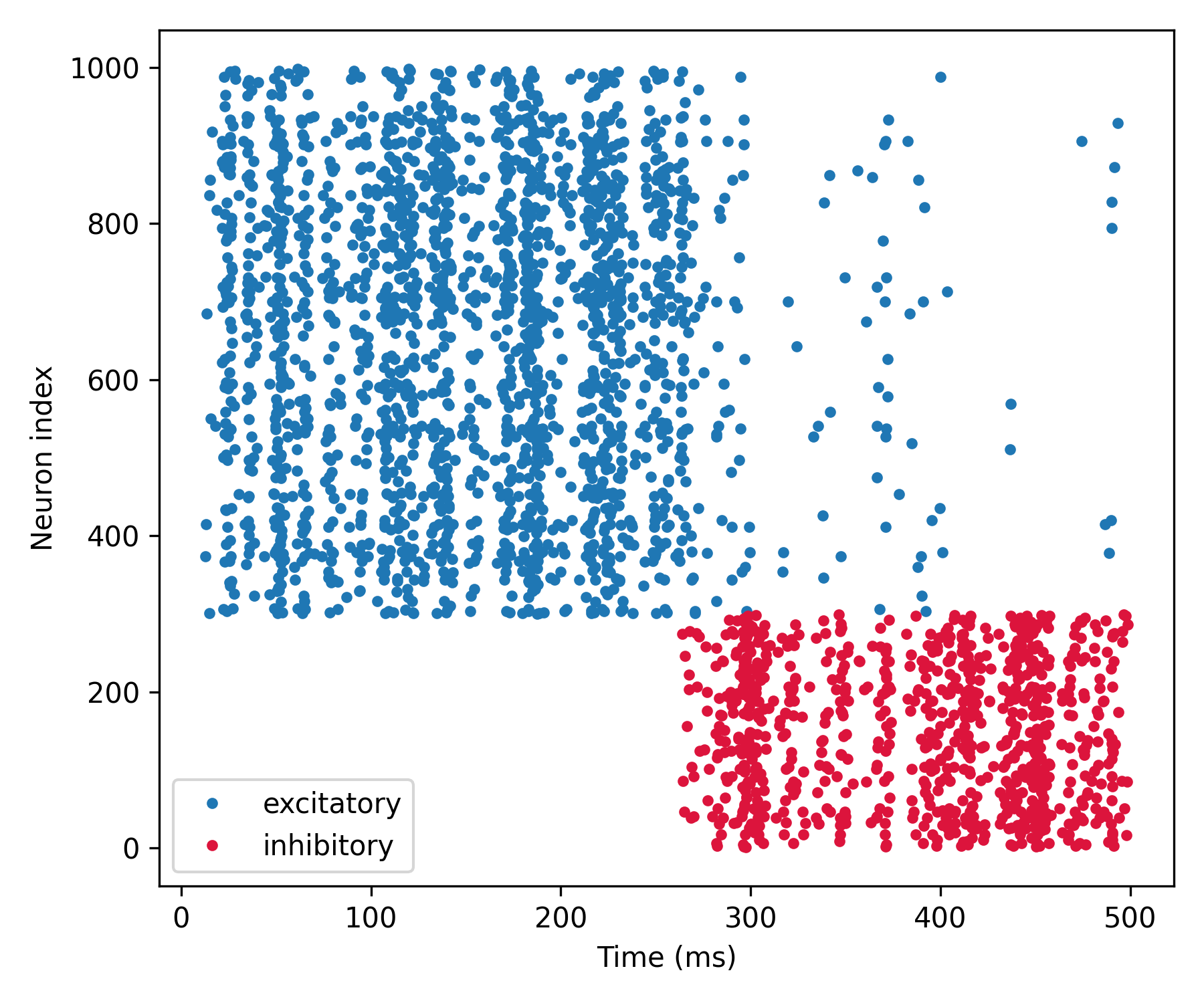
N_e = 700
N_i = 300

# Create a neuron model
model = PointNeuronModel(model='leakyIF', cm_abs=281*pF, gl_abs=30*nS,
                         v_rest=-70.6*mV)

# external excitatory input
model.synapse('AMPA', tag='ext', g=2*nS, t_decay=2.5*ms)
model.synapse('GABA', tag='inh', g=2*nS, t_decay=7.5*ms)  # feedback inhibition
model.add_params({'Vth': -40.4*mV, 'Vr': -65.6*mV})

# Create a NeuronGroup
neurons = model.make_neurongroup(N=N_e+N_i, threshold='V>Vth',
                                 reset='V=Vr', method='euler')

# Subpopulation of 300 inhibitory neurons
inhibitory = neurons[:N_i]

# Subpopulation of 700 excitatory neurons
excitatory = neurons[N_i:]

# Create a Poisson input
Input = b.PoissonGroup(200, rates=90*Hz)

# Specify synaptic connections
Syn_ext_a = b.Synapses(Input, excitatory, on_pre='s_AMPA_ext += 1')
Syn_ext_a.connect(p=0.2)

Syn_ext_b = b.Synapses(Input, inhibitory, on_pre='s_AMPA_ext += 1')
Syn_ext_b.connect(p=0)  # initially no connections to inhibitory neurons

Syn_inh = b.Synapses(inhibitory, excitatory, on_pre='s_GABA_inh += 1')
Syn_inh.connect(p=0.15)

# Record voltages and spike times
spikes_e = b.SpikeMonitor(excitatory)
spikes_i = b.SpikeMonitor(inhibitory)

# Run simulation
b.run(250 * ms)
Syn_ext_b.connect(p=0.2)  # add connections to inhibitory neurons
b.run(250 * ms)

# Plot results
b.figure(figsize=[6, 5])
b.plot(spikes_e.t/ms, spikes_e.i+N_i, '.', label='excitatory')
b.plot(spikes_i.t/ms, spikes_i.i, '.', label='inhibitory', c='crimson')
b.xlabel('Time (ms)')
b.ylabel('Neuron index')
b.legend()
b.tight_layout()
b.show()