Membrane time constant
In this example, we show how to calculate a neuron’s membrane time constant
τm, a metric that describes how quickly the membrane potential V decays
to its steady-state value after some perturbation. In simple RC circuits, τm
is calculated as the product of the membrane capacitance C and the membrane
resistance R. However, in neurons, τm is also affected by voltage-gated
conductances or other non-linearities.
Experimentally, τm is often calculated by fitting an exponential function to
the membrane potential V trace after applying a small negative current pulse
at rest.
Here we explore:
How to calculate
τmfor a neuron model experimentally.How
τmis affected by the presence of voltage-gated conductances, such as an adaptation current.
import brian2 as b
from brian2.units import ms, mV, nS, pA, pF
from scipy.optimize import curve_fit
from dendrify import PointNeuronModel
b.prefs.codegen.target = 'numpy' # faster for simple simulations
# Create neuron models
GL = 20*nS # membrane leak conductance
CM = 250*pF # membrane capacitance
EL = -70*mV # resting potential
tau_theory = CM / GL # theoretical membrane time constant
lif = PointNeuronModel(model='leakyIF', cm_abs=CM, gl_abs=GL, v_rest=EL)
aif = PointNeuronModel(model='adaptiveIF', cm_abs=CM, gl_abs=GL, v_rest=EL)
aif.add_params({'tauw': 100*ms, 'a': 2*nS})
# Create NeuronGroups (no threshold or reset conditions for simplicity)
lif_neuron = lif.make_neurongroup(N=1, method='euler')
aif_neuron = aif.make_neurongroup(N=1, method='euler')
# Record voltages
lif_monitor = b.StateMonitor(lif_neuron, 'V', record=0)
aif_monitor = b.StateMonitor(aif_neuron, 'V', record=0)
# Run simulation
I = -10*pA # current pulse amplitude
t0 = 20*ms # time to start current pulse
t_stim = 200*ms # duration of current pulse
b.run(t0)
lif_neuron.I_ext, aif_neuron.I_ext = I, I
b.run(t_stim)
lif_neuron.I_ext, aif_neuron.I_ext = 0*pA, 0*pA
b.run(100*ms)
# Analysis code
def func(t, a, tau):
"""Exponential decay function"""
return a * b.exp(-t / tau)
def get_tau(trace, t0):
dt = b.defaultclock.dt
Vmin = min(trace)
time_to_peak = list(trace).index(Vmin)
# Find voltage from current-start to min value
voltages = trace[int(t0/dt): time_to_peak] / mV
# Min-max normalize voltages
v_norm = (voltages - voltages.min()) / (voltages.max() - voltages.min())
# Fit exp decay function to normalized data
X = b.arange(0, len(v_norm)) * dt / ms
popt, _ = curve_fit(func, X, v_norm)
return popt, X, v_norm
# Plot results
popt_lif, X_lif, v_norm_lif = get_tau(lif_monitor.V[0], t0)
popt_aif, X_aif, v_norm_aif = get_tau(aif_monitor.V[0], t0)
fig, axes = b.subplot_mosaic("""
AA
BC
""", layout='constrained', figsize=[6, 5])
ax0, ax1, ax2 = axes.values()
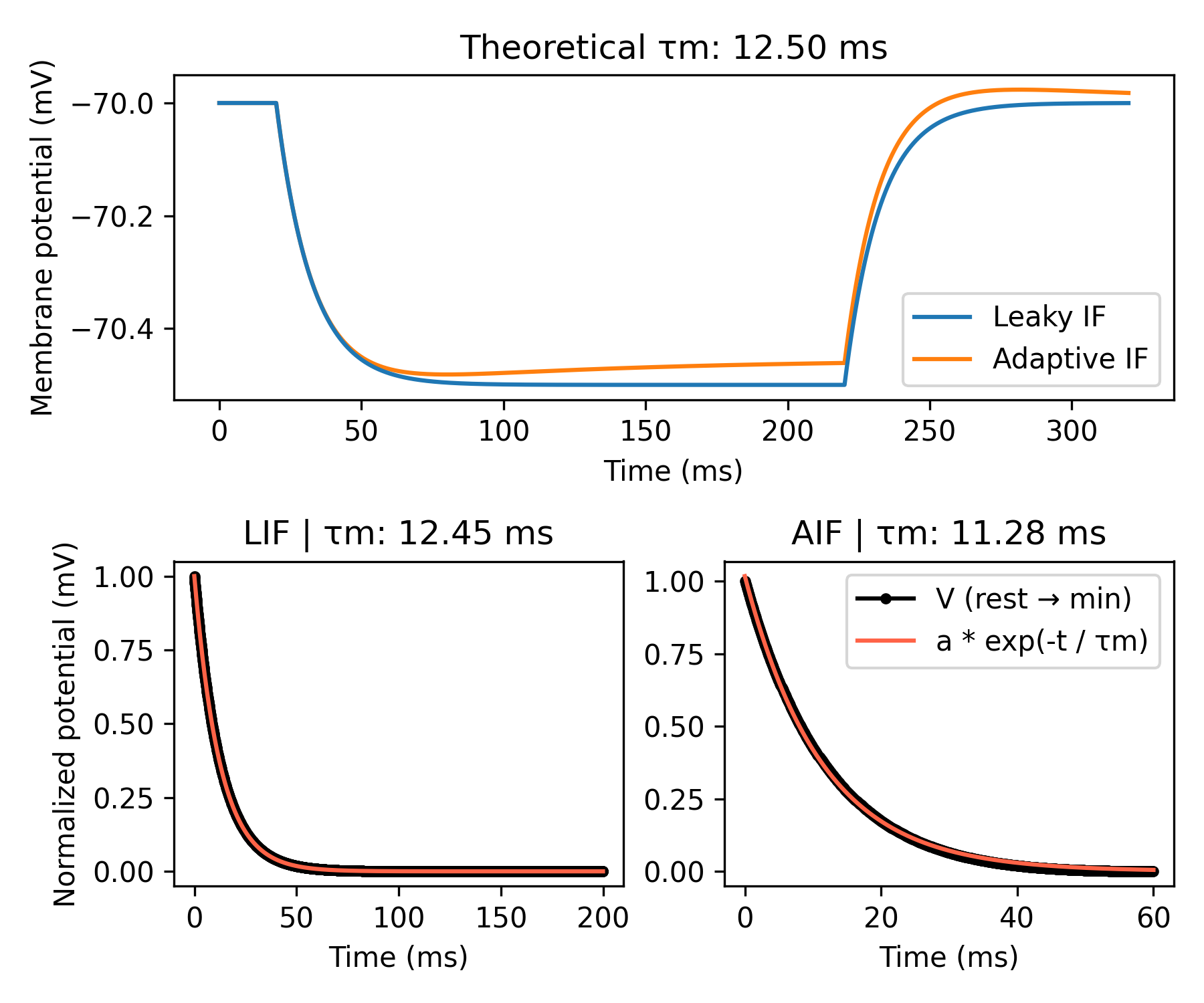
ax0.plot(lif_monitor.t/ms, lif_monitor.V[0]/mV, label='Leaky IF')
ax0.plot(aif_monitor.t/ms, aif_monitor.V[0]/mV, label='Adaptive IF', zorder=0)
ax0.set_title('Theoretical τm: {:.2f} ms'.format(tau_theory/ms))
ax0.set_ylabel('Membrane potential (mV)')
ax0.legend()
ax1.plot(X_lif, v_norm_lif, 'ko-', ms=3)
ax1.plot(X_lif, func(X_lif, *popt_lif), c='tomato')
ax1.set_ylabel('Normalized potential (mV)')
ax1.set_title(f'LIF | τm: {popt_lif[1]:.2f} ms')
ax2.plot(X_aif, v_norm_aif, 'ko-', label='V (rest \u2192 min)', ms=3)
ax2.plot(X_aif, func(X_aif, *popt_aif), label='a * exp(-t / τm)', c='tomato')
ax2.set_title(f'AIF | τm: {popt_aif[1]:.2f} ms')
ax2.legend()
for ax in axes.values():
ax.set_xlabel('Time (ms)')
fig.tight_layout()
b.show()